Multiples, Models and Metrics
.
| Single-Stage Valuation Multiples | Multi-Stage Valuation Multiples | g Solution |
| Observed Multiples | Target Multiples |
Single-Stage Valuation Multiples1
A valuation multiple is simply a ratio through which we view the value of the firm as a function of one if its inputs. These ratios, most often a quotient including some notion of the firm’s value interacted with an income based variable, offer a comparative metric useful for many reasons, not the least being a sense of the firm’s relative position among a group of peers. While on the surface this may appear to be more about a comparative metric, what underlies the ratio, or multiple, is a complex series of calculations and outcomes informing knowledgeable investors and analysts of the firm’s value.
Applying a single-stage multiple is simple and observable. We’ll use an EV/FCF model as an example.

For the left hand side of this equation we use the firm’s observable Enterprise Value at a particular point in time and divide that value by the firm’s Free Cash Flow as of the same point in time, resulting in some multiple value for the left side of the equation. The right side of the equation is somewhat more complex and relies on the use of the firm’s Return on Invested Capital (ROIC), Weighted Average Cost of Capital (WACC), expected growth rate and tax rate on EBIT for the same point in time.
A single-stage multiple’s virtue is in its simplicity. A single-stage multiple’s vice is similarly in its simplifying assumptions. However, it is an interesting tool and has credible utility when used appropriately, such as in a multi-stage valuation model or an attempt at solving for the g solution or market’s inferred growth rate for the subject firm.
1Richard Haskell, PhD (2017), Associate Professor of Finance, Bill & Vieve Gore School of Business, Westminster College, Salt Lake City, Utah, rhaskell@westminstercollege.edu, www.richardhaskell.net.
A Single-Stage Multiple in a Multi-Stage Valuation Model1
In a two-stage valuation model, the single-stage multiple is simplified and rearranged to solve for EV by multiplying both side by the cash flow variable:

In this form, the multiple acts as a continuing (terminal) value and is likely the result of a future forecasted cash flow multiplied by a target multiple which can then be discounted for time to the present resulting in a present value of the continuation value (PVCV)
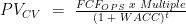
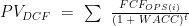
This can be added to the explicit forecast period of the two-stage valuation model which is the discounted present value of the subject cash flow (PVDCF)
The two stages can then be added to form a multi-stage valuation model using a single–stage valuation multiple for its terminal value

In the model’s first stage the cash flows being summed are likely the result of financial forecasting of the firm’s expected incomes and expenses for the explicit period. In the model’s second stage the growth rate of the cash flow is held constant in perpetuity.
1Richard Haskell, PhD (2017), Associate Professor of Finance, Bill & Vieve Gore School of Business, Westminster College, Salt Lake City, Utah, rhaskell@westminstercollege.edu, www.richardhaskell.net.
Multi-Stage Valuation Multiples1
A multi-stage valuation multiple relaxes the constraining assumptions used in a single-state multiple and extends the multiple to multiple periods of time, each with potentially unique rates of growth (g) and WACC. It also assumes that ROIC is equal to WACC in the continuation period (perpetuity).
![\frac{EV}{FCF_{OPS}}\,\,=\,\,\frac{ROIC\,\,-\,\,g}{ROIC\,\,(WACC\,\,-\,\,g)}\,\,(1\,\,-\,\,T)\,\,x\,\,\big[1\,\,-\,\,\frac{(1\,\,+\,\,g)^{n}}{(1\,\,+\,\,WACC)^{n}}\big])\,\,+\,\,\frac{1}{WACC}\,\,x\,\,\frac{(1\,\,+\,\,g)^{n}}{(1\,\,+\,\,WACC)^{n}}](http://s0.wp.com/latex.php?latex=%5Cfrac%7BEV%7D%7BFCF_%7BOPS%7D%7D%5C%2C%5C%2C%3D%5C%2C%5C%2C%5Cfrac%7BROIC%5C%2C%5C%2C-%5C%2C%5C%2Cg%7D%7BROIC%5C%2C%5C%2C%28WACC%5C%2C%5C%2C-%5C%2C%5C%2Cg%29%7D%5C%2C%5C%2C%281%5C%2C%5C%2C-%5C%2C%5C%2CT%29%5C%2C%5C%2Cx%5C%2C%5C%2C%5Cbig%5B1%5C%2C%5C%2C-%5C%2C%5C%2C%5Cfrac%7B%281%5C%2C%5C%2C%2B%5C%2C%5C%2Cg%29%5E%7Bn%7D%7D%7B%281%5C%2C%5C%2C%2B%5C%2C%5C%2CWACC%29%5E%7Bn%7D%7D%5Cbig%5D%29%5C%2C%5C%2C%2B%5C%2C%5C%2C%5Cfrac%7B1%7D%7BWACC%7D%5C%2C%5C%2Cx%5C%2C%5C%2C%5Cfrac%7B%281%5C%2C%5C%2C%2B%5C%2C%5C%2Cg%29%5E%7Bn%7D%7D%7B%281%5C%2C%5C%2C%2B%5C%2C%5C%2CWACC%29%5E%7Bn%7D%7D&bg=ffffff&fg=000&s=0&c=20201002)
The strength of a multi-stage multiple is in its allowance for different rates of growth and WACC in the continuation period. A potential weakness of this particular form is that it operates under the assumption that there is no value added in the continuation period; that is, ROIC is equal to WACC such that continued growth does not add value to the firm.
We can relax the model’s assumptions further supposing the firm does add value in the continuation period by differentiating the firm’s expected long-term (LT) returns and cost costs of capital
![\frac{EV}{FCF_{OPS}}\,\,=\,\,\frac{ROIC\,\,-\,\,g}{ROIC\,\,(WACC\,\,-\,\,g)}\,\,(1\,\,-\,\,T)\,\,x\,\,\big[1\,\,-\,\,\frac{(1\,\,+\,\,g)^{n}}{(1\,\,+\,\,WACC)^{n}}\big])\,\,+\,\,\frac{ROIC_{LT}\,\,-\,\,g_{LT}}{ROIC_{LT}\,\,x\,\,(WACC_{LT}\,\,-\,\,g_{LT})}\,\,x\,\,\frac{(1\,\,+\,\,g)^{n}}{(1\,\,+\,\,WACC)^{n}}](http://s0.wp.com/latex.php?latex=%5Cfrac%7BEV%7D%7BFCF_%7BOPS%7D%7D%5C%2C%5C%2C%3D%5C%2C%5C%2C%5Cfrac%7BROIC%5C%2C%5C%2C-%5C%2C%5C%2Cg%7D%7BROIC%5C%2C%5C%2C%28WACC%5C%2C%5C%2C-%5C%2C%5C%2Cg%29%7D%5C%2C%5C%2C%281%5C%2C%5C%2C-%5C%2C%5C%2CT%29%5C%2C%5C%2Cx%5C%2C%5C%2C%5Cbig%5B1%5C%2C%5C%2C-%5C%2C%5C%2C%5Cfrac%7B%281%5C%2C%5C%2C%2B%5C%2C%5C%2Cg%29%5E%7Bn%7D%7D%7B%281%5C%2C%5C%2C%2B%5C%2C%5C%2CWACC%29%5E%7Bn%7D%7D%5Cbig%5D%29%5C%2C%5C%2C%2B%5C%2C%5C%2C%5Cfrac%7BROIC_%7BLT%7D%5C%2C%5C%2C-%5C%2C%5C%2Cg_%7BLT%7D%7D%7BROIC_%7BLT%7D%5C%2C%5C%2Cx%5C%2C%5C%2C%28WACC_%7BLT%7D%5C%2C%5C%2C-%5C%2C%5C%2Cg_%7BLT%7D%29%7D%5C%2C%5C%2Cx%5C%2C%5C%2C%5Cfrac%7B%281%5C%2C%5C%2C%2B%5C%2C%5C%2Cg%29%5E%7Bn%7D%7D%7B%281%5C%2C%5C%2C%2B%5C%2C%5C%2CWACC%29%5E%7Bn%7D%7D&bg=ffffff&fg=000&s=0&c=20201002)
While a multi-stage model in which rates of growth, ROIC, and WACC can be differentiated yields interesting results, its use warrants a note of caution:
- Absent some product or process innovation in which the firm continues to wield a competitive advantage over its industry peers, there is no expected gain in the long-term beyond that which the expected cost of capital captures
- Valuation equations in which a substantial spread between long-term returns and costs of capital are forecast often result in unrealistically high outcomes
- Perpetuity is a long time and there are no known examples of firms maintaining such an advantage in the long-run.
1Richard Haskell, PhD (2017), Associate Professor of Finance, Bill & Vieve Gore School of Business, Westminster College, Salt Lake City, Utah, rhaskell@westminstercollege.edu, www.richardhaskell.net.
g Solution1
Though EV/EBIT is a metric with an observable value and can be rearranged into a simplified valuation models, it also has significant additional potential. Like most multiples it can be expressed algebraically using additional firm level inputs for Return on Invested Capital (ROIC), Weighted Average Cost of Capital (WACC), expected growth (g) and average tax rate on EBIT (T). When these inputs include time signatures in which t = 0 is the point of observation and t > 0 is some future point in time, the EV/EBIT equation can be rewritten as follows:

The right hand side of this equation may be used to shed some light on how the markets perceive the growth prospects of the firm. Given that a market-based EV is informed by exchange transactions we can infer the market’s consensus of g by using observed values for EV, EBIT, ROIC, WACC and T and solving for this market inferred g:
Start by dividing both sides of the equation by the denominators and substituting T’ for (1-T):
![(EV_{0})\big[ROIC_{0}(WACC_{0}\,\,-\,\,g)\big]\,\,=\,\,(ROIC_{0}\,\,-\,\,g)\,(T')\,(EBIT_{0})](http://s0.wp.com/latex.php?latex=+%28EV_%7B0%7D%29%5Cbig%5BROIC_%7B0%7D%28WACC_%7B0%7D%5C%2C%5C%2C-%5C%2C%5C%2Cg%29%5Cbig%5D%5C%2C%5C%2C%3D%5C%2C%5C%2C%28ROIC_%7B0%7D%5C%2C%5C%2C-%5C%2C%5C%2Cg%29%5C%2C%28T%27%29%5C%2C%28EBIT_%7B0%7D%29&bg=ffffff&fg=000&s=0&c=20201002)
Expand each side of the equation:

Rearrange to include all g terms on the right

Factor out g and ROIC0
![g\, \big[(T')(EBIT_{0})\,\,-\,\,(EV_{0})(ROIC_{0})\big]\,\,=\,\,ROIC_{0}\,\big[(T')(EBIT_{0})\,\,-\,\,(EV_{0})(WACC_{0})\big]](http://s0.wp.com/latex.php?latex=+g%5C%2C+%5Cbig%5B%28T%27%29%28EBIT_%7B0%7D%29%5C%2C%5C%2C-%5C%2C%5C%2C%28EV_%7B0%7D%29%28ROIC_%7B0%7D%29%5Cbig%5D%5C%2C%5C%2C%3D%5C%2C%5C%2CROIC_%7B0%7D%5C%2C%5Cbig%5B%28T%27%29%28EBIT_%7B0%7D%29%5C%2C%5C%2C-%5C%2C%5C%2C%28EV_%7B0%7D%29%28WACC_%7B0%7D%29%5Cbig%5D&bg=ffffff&fg=000&s=0&c=20201002)
Divide both sides by to arrive at g solution
![g\,\,=\,\,\frac{ROIC_{0}\,\big[(T')(EBIT_{0})\,\,-\,\,(EV_{0})(WACC_{0})\big]}{ (T')(EBIT_{0})\,\,-\,\,(EV_{0})(ROIC_{0})}](http://s0.wp.com/latex.php?latex=+g%5C%2C%5C%2C%3D%5C%2C%5C%2C%5Cfrac%7BROIC_%7B0%7D%5C%2C%5Cbig%5B%28T%27%29%28EBIT_%7B0%7D%29%5C%2C%5C%2C-%5C%2C%5C%2C%28EV_%7B0%7D%29%28WACC_%7B0%7D%29%5Cbig%5D%7D%7B+%28T%27%29%28EBIT_%7B0%7D%29%5C%2C%5C%2C-%5C%2C%5C%2C%28EV_%7B0%7D%29%28ROIC_%7B0%7D%29%7D&bg=ffffff&fg=000&s=0&c=20201002)
Knowing the growth (g) the market projects for the firm allows us to make a more informed investment decision: if g is greater than might be reasonably expected then, the firm might warrant a sell recommendation; if g is less then perhaps a buying opportunity is being presented.
Also, if we forecast future changes in ROIC and WACC we can return to the consideration of the EV/EBIT multiple as a valuation model using the market inferred g by substituting expected values for EBIT, ROIC and WACC into the equation and solving for some future value of EV:
So, a valuation multiple is much more than simply a quotient or comparative ratio. In the hands of a creative and informed analyst it becomes a multipurpose tool capable of informing expected values for a firm, inferring a consensus rate of growth for the subject firm, or even predicting and confirming an appropriate level for a target valuation multiple.
When the growth rate of a firm’s cash flow variable is expected to remain constant over time, a relatively unrealistic expectation, a single-stage valuation multiple similar to the EV/EBIT multiple form noted. However, when forecast values of a firm’s cash flow variable are not expected to be constant a two-stage multiple construction may be useful; a form capable of assessing a period during which the growth rate of the cash flow is non-constant followed by a continuation period during which the rate is held constant. Given that accurately forecasted cash flows become increasingly unlikely as the forecast period becomes lengthy, two-stage multiples are commonly applied, as are two stage valuation models in which a single stage valuation multiple is used to form the firm’s continuation value (terminal value).
The dynamics of valuation multiples are such that they may be readily observed, as noted, formed as a target multiple, or abstractly conceptualized as a multiple with some theoretical value. The multipurpose valuation multiples includes each.
1Richard Haskell, PhD (2017), Associate Professor of Finance, Bill & Vieve Gore School of Business, Westminster College, Salt Lake City, Utah, rhaskell@westminstercollege.edu, www.richardhaskell.net.
Observed Multiples1
Enterprise and Equity valuation multiples are observable values based on the market value of the firm’s underlying equity and debt capital less cash and equivalents, or Enterprise Value (EV), as interacted with the selected variable (EBIT, EBITDA, NOPLAT, FCF, IC) as a quotient. The firm’s EV is set by exchanges in the market effected by substantial numbers of economic agents providing bid and ask pricing for the subject equity and debt instruments. The variable against which EV is interacted is simply an accounting identity and measurable through the firm’s income statement and/or balance sheet as reported. With this known or observed value for the subject multiple, investors, analysts, and firm managers may compare one firm’s performance against another, consider possible changes in value based on presumed changes in the accounting identity, or possibly predict a market inferred value for one of the multiple’s input components such as ROIC, WACC or g.
The observable multiple forms under consideration in this study include
1Richard Haskell, PhD (2017), Associate Professor of Finance, Bill & Vieve Gore School of Business, Westminster College, Salt Lake City, Utah, rhaskell@westminstercollege.edu, www.richardhaskell.net.
Target Multiples1
While an Observed Multiples reflects a specific market value and accounting identity for a subject firm, a Target Multiple is aspirational and is typically formed through one of a limited number of methods:
- Examination of of Public Comparables or Precedent Transactions
- Examination of observed historic multiple values
- An an algebraic equivalent to the observed multiple
While considerate of the various means of establishing a Target Multiple, this study concentrates on the an algebraic equivalent to the observed multiple itself. In so doing, we gain insights into what a subject firm’s multiple values might be given a set on inputs. Considering a target multiple in this manner may also assist in solving for one of these variable when taking the observed multiple value as given.
The right hand term in the following multiple equations represent those Single-Stage Target Multiple equations under consideration in this study and allow for the use of the valuation multiple as a predictive tool:
| Enterprise Multiples | ||
| EV/SALES | 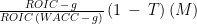 |
|
| EV/EBIT | 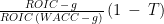 |
|
| EV/NOPLAT | 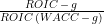 |
|
| EV/EBITDA | 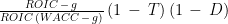 |
|
| EV/FCFOPS | |
|
| EV/IC |  |
|
| Equity Multiples | ||
| PRICE/EARNINGS | 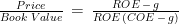 |
|
| PRICE/BOOK VALUE | 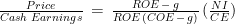 |
|
| PRICE/CASH EARNINGS |  |
|
1Richard Haskell, PhD (2017), Associate Professor of Finance, Bill & Vieve Gore School of Business, Westminster College, Salt Lake City, Utah, rhaskell@westminstercollege.edu, www.richardhaskell.net.